What is the Quality of Data?

We work hard to provide accurate data to you the end user, and have a lot of confidence in our methodology. But with any data, users should be aware of innacuracies that may occur and caveats that you should hold when viewing data.

Fleet Sizes and Search Horizons

In the world of shared mobility, fleets are managed by operators, who make these vehicles available for use by the general public. These vehicles can be owned and maintained by operators (as in most scooter companies), or owned independently but managed through a platform (for example, many ride-hailing services).

The fleet size is an incredibly important metric, as it tells a city how many devices an operator has. Many permit or license requirements include limits on the maximum fleet a single operator can have, known as a fleet cap (the opposite, a minimum number of devices an operator is required to have, is known as a fleet floor). Knowing the size of the fleet helps cities understand whether there are too few, too many, or just the right number of devices for their needs.

Vianova defines Fleet Size as "The best estimate of the number of vehicles currently in the public right-of-way (PROW) at a given time." We intentionally omit vehicles not on the public right-of-way (e.g., vehicles stored in the warehouse). However, we include vehicles that are in the public right-of-way but unavailable for rental (more on this later).

Fleet size is an instantaneous KPI, changing many times in a single hour. To simplify analysis, we take a snapshot of the fleet at the top of every hour, exactly after the hour changes. Any vehicle that is not in state RM (ref: device states) is counted towards fleet size.

The daily average fleet size is the sum of all hourly fleet sizes, divided by 24. The weekly average fleet size is the sum of all daily average fleet sizes in that week, divided by 168 (24 hours multiplied by 7 days). For any period, the average fleet size is the sum of the hourly fleet sizes, divided by the number of hours in the period.

Different cities apply fleet sizes in different ways. Some cities elect to use a daily (or weekly or monthly) average, while others take the fleet size from the largest single hour (or day or week). Both calculations are valid, it is ultimately a policy question that a city can decide on.

Limitations and Search Horizons

By design, MDS is not designed to provide the state of a single device at a given time. So if you want to know what the current status of a particular device is, you need to look for the latest known state of this device by looking at the historical collections of events from the Provider API. That's what we call internally the "search horizon". The devices whose last status change was within that search horizon are presumed to still be on the street, and therefore counted as part of the fleet size in the hourly snapshots.

One of the major concerns related to this limitation is the capacity to have a clear picture of the current fleet size at a particular moment. In the example below, you will better understand why adjusting the "search horizon" can have a real impact on how many devices are included in the fleet size calculation.

In this scenario, let's consider 4 different devices, that are made Available (AV),

but not at the same time. A device is made available when it finishes a trip or is put back into service after having been taken offline by a company.

Device A has become Available within the last 24 hours

Device B has become Available within the last 72 hours

Device C has become Available within the last week

Device D has become Available within the last 48 hours

Depending on what "search horizon", we use, we could wind up with 1, 2, 3, or 4 devices in the fleet.

At Vianova, we believe that the best "search horizon" for vehicle state is 7 days, which we have revised upward from 4 days in our product updates as of April, 2021. This number represents the best representation of the situation on the ground, and encourages operators to make sure that their devices are positioned such that they are being used.

What's next

In the near future we will provide cities the ability to set their own search horizons. For a range of reasons, cities may elect to have shorter search horizons, though we will continue to use a default of 7 days.

It's part of our job to continue improving our analytics to be as close as possible to reality, so we can better help cities to make the right decisions.

Important considerations

The hourly fleet size is the instantaneous value at the top of the hour

The daily fleet size is the average of the 24 values of each hours of the day

Timestamps from the API are provided in ISO Format, with Timezone information included

Event Statuses

Each operator is responsible for transmitting data via MDS and GBFS to Vianova, which aggregates that data and layers on an additional set of tools to help you derive insight and intelligence from the data. However, most operators are not using MDS statuses to manage their own internal operations, but rather use their own fleet management tools.

The data in these fleet management tools is "mapped" to MDS, so that the words or statuses that a company uses to describe its own data internally are "translated" into the standard language used by MDS. However, sometimes errors in this translation can occur, and the data can misrepresent the status on the ground.

GPS and Vehicle Positioning

The positioning of a parked device is provided as a set of GPS coordinates. This position is derived primarily from the cellular connection on a vehicle. As with any GPS, the accuracy of this position can be affected by several factors, including the height and material of nearby buildings, the quality of the GPS hardware, weather conditions, and other data. Because of these errors different operators and different cities can have different GPS inaccuracies. It is not uncommon for devices to have GPS errors of 5-10 meters from where Cityscope identifies them.

Telemetries and Moving Vehicle Data

In the world of connected vehicles, there is an important concept called "telemetries". It's basically the way a device collects, stores, and exposes some geographical information. You can think of this as the device reporting timestamped updates of its current position (and other device-properties) to some server. Typically, the device is programmed to record its position at regular intervals (say, every 10 seconds), which we call the "sampling rate".

Connected vehicles have GPS hardware embedded to track their position so the fleet managers know where the device is for important reasons like:

the device is low on battery
the device requires maintenance
the device has left the proper operating zone,

Those telemetries are then stored in the provider's fleet management system and could be exposed to other 3rd parties like Vianova through the MDS API trips endpoint.

The GBFS specification only exposes information about parked devices. To extract trip information, we need to track when a parked vehicle "reappears" in a new location after a certain period of time has elapsed. Thus, it's clear that the best one can do with GBFS is extract only the start and end position of "potential" trips.

In contrast, the MDS specification requires that at a minimum the provider should expose the first and the last point (aka start of trip position and end of trip position).

Based on Vianova's experience in managing shared mobility data, we have determined that 6 telemetries per minute is an acceptable rate of telemetries to enable Vianova to fulfil the use cases laid out by cities. It is particularly important for mapping trips to street segments and aggregating them over time, in order to reflect the number trips/days across the whole city for each street.

Our goal is to better map street segment usage, so the city can better understand and prioritise transportation investments. Knowing that a street is frequently used could lead to a decision of the creation of a bike lane or better turning infrastructure, for example.

Parked Vehicle Positions

Cityscope uses the "Event Location" field of MDS Provider to position a device that is not on a trip. The last event of a device represents the reported location of a trip end, an operator drop off, etc. This position may vary slightly from the current position of the device as a result of the reliance on the single GPS observation of the point. The vehicle's position is not updated until a new event (such as a user trip start or an operator pick-up) is triggered.

Data coming from other sources which update independently of vehicle events (such as GBFS or MDS Agency) may result in different locations for the vehicle in "real-time". Our decision to use MDS Provider reflects the most standardized response to the differences in data quality and availability among the providers operating in different cities.

Trip Distances

The length of a shared mobility trip is a very important measure. It helps to answer questions about whether shared mobility is replacing public transport or vehicle trips, allows for calculations of speed, and enables calculations about the greenhouse gas emissions of shared mobility per kilometer.

The distance between an origin and a destination can be reported two ways. The first is the crow-flies distance, which represents a straight line between the origin and destination (the shortest distance). The second reporting is a on-road distance, which represents the twists and turns that are necessary on the ground in order to get between the origin and destination. Many factors can contribute to the difference between crow-flies and on-road distances such as the complexity of the street grid, the location of infrastructure such as cycle paths, the weather, and even the price to rent devices.

Different shared mobility operators report distance in different ways. Several operators provide the on-road distance between the origin and destination, backed up by a series of mid-trip telemetries (essentially GPS locations every few seconds along the route of the trip). Other operators provide on-road distances, but no mid-trip telemetries. And finally, some operators only provide crow-flies distances, computed based solely on the locations of the origins and destinations. For more information about telemetries, see this article.

This table shows a range of providers we have worked with across several cities. If "100" represents a crow-flies distance, the actual distance we receive ranges from 100 (ie, we only receive crow-flies distance) to more than twice that length in on-road distance.

Comparing or averaging crow-flies and on-road distances together is a bad practice, because they are two different measures. In order to approximate the on-road distance when only crow-flies is available, Vianova multiplies all crow-flies distances by a factor of 1.5. This number reflects the most common difference between crow-flies and on-road distances and allows for more meaningful analytics, although it should be considered an estimate. As operators improve the distances they report, we can gradually replace all crow-flies distances with more accurate on-road conditions.

Zone Buffering and GPS Accuracy

Generally, within Cityscope, a user has two ways of interacting with a contextual zone (i.e.: your entire operational area). One can either:

gather analytics of travel patterns or usage in a particular area
create a regulation to collect infringements for a particular area

In both cases, it is useful to augment the geographical region with a buffer to better target the user's intent.

Analytics
"Analytics" means the review of data to understand usage patterns and behaviours. As there is not typically a regulatory use of analytics, Vianova recommends using a wide buffer to account for issues with the accuracy of on-device GPS. We have calculated that adding a 10 meter positive buffer (ie, a perimeter extending 10 meters beyond the drawn boundary) produces the best results, for two reasons :

mobility hubs are typically drawn quite small (frequently under 10 meters square) and as a result, sometimes devices are parked in the hub but not correctly located as a result of GPS inaccuracy.

GPS imprecision may lead to an up to 5m error of the digital policy when compared to the real physical coordinates. As a result, only counting devices in the digital policy can exclude correctly parked vehicles. This issue is exacerbated when the geography is small.

Regulation

In the case of a regulation (such as a no parking zone), the approach is similar, but the inverse applies. Because devices are typically parked at the edge of the regulated zone, GPS inaccuracy will again include them and they will be reported in infractions. So the closer we get to the heart of the zone (see matching), the greater our confidence that the device is truly in violation of a No Parking Zone policy as shown in this example.

Accounting for this GPS inaccuracy, we have introduced this notion of "Confidence level" based on the number of meters that the device is from the actual border of the geometry.

In order to improve the quality of the reporting, Vianova has reviewed over 100k infractions. As you can see in the chart below, the vast majority of infractions occur within the first 9 meters of the border of a no parking zone. In order to ensure that an automated violation on Cityscope reflects the on the ground reality, a negative buffer is used to separate the vehicles the system is Confident in from those devices that are merely Likely or Possibly in violation. Since violations may have financial penalties on operators, it is important to distinguish the violations that we are almost certainly accurate from those which may require visual inspection to confirm. These Likely or Possible violations are still important for the city to consider, and they suggest where the city may wish to deploy inspectors or parking enforcement officers.

Based on the data Vianova has analysed, we advise cities to consider using a 7 meters negative buffer as the correct amount to reach an appropriately Confident level that the violation is accurate.

We will continue evaluating ways to improve the buffers on our policies. As the accuracy of device GPS improves, as well as our methods for determining true ground positions, we will modify the buffers in order to better reflect the real world.

K-Anonymization

K-anonymization is the approach Vianova takes to avoid exposing non-aggregated data. We don’t want to be able to identify individuals who have made trips to specific locations. In order to achieve this goal, we won’t expose data where the trip counts is less than a given threshold. Vianova has set that threshold by default as k=3. This may mean that some data may appear to not add up- for example, if you break down the number of devices in a City into its subdistricts, the sum of the subdistricts will likely be lower than the total for the city, as we are not displaying subdistricts with 1 or 2 devices.

When the riding count is < k, we won’t expose :

The riding count

When the origin count is < k, we won’t expose :

The origin count
The origin distance
The origin duration
The vehicle rotation

When the destination count is < k, we won’t expose :

The destination count
The destination distance
The destination duration

Review the metrics dictionary for the specific definition of these terms.

Finding Historic Data

When we start working with a new city or a new operator, we will automatically attempt to "backfill" historic data so that someone can see what was happening in the past, even prior to today. A backfill relies on the feed providers retaining information about past events in the feed for some historic period of time, so that the history can be reconstructed. We may encounter limits to the backfill such as:

An operator not retaining any historic data in their feed
An operator delivering data for a fixed amount of time (ie, just the past three months)
An operator changing their MDS feed versions
An operator restricting our access to historic data

If you believe that historic data exists but is not showing on the platform, let us know and we can discuss opportunities with the operator to reconstruct the timeline.

Map Views and Data Sampling

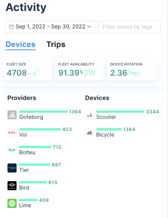
When on the Activity Page, you may notice that information on the left-hand side of the page does not line up precisely to the information on the map itself. This is due to the different approaches we take to producing metrics (the graphs and tables you see) and visualizations (the map).

Metrics are always true and accurate information produced to the best of our ability. The image below represents the average fleet size, fleet availability, and device rotation for an hour during the period of September 1 through September 30, 2022. This number can be calculated based on the metrics computations which we run each hour, a total of 720 observations over this month.

In contrast, visualizations on the map are representative of the period in question. It is not possible to display on a map the physical position of every device at every moment in the monthlong period. So Cityscope uses a set of samples in order to produce a map representing the most likely device positions (or trip starts or ends, in the case of trips) over the period in question.

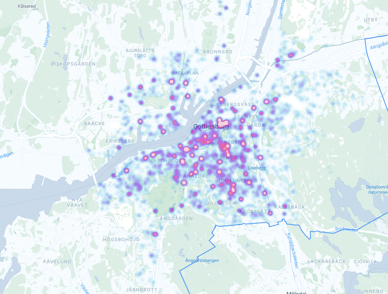
Heat Maps

Heat maps are a simple visual to understand the relative density of points. Cityscope takes a random sample of no more than 15,000 events occurring in the period (vehicle positions, trip starts, trip ends) and displays them on the map- the areas with higher intensities are the places where the number of events are greater.

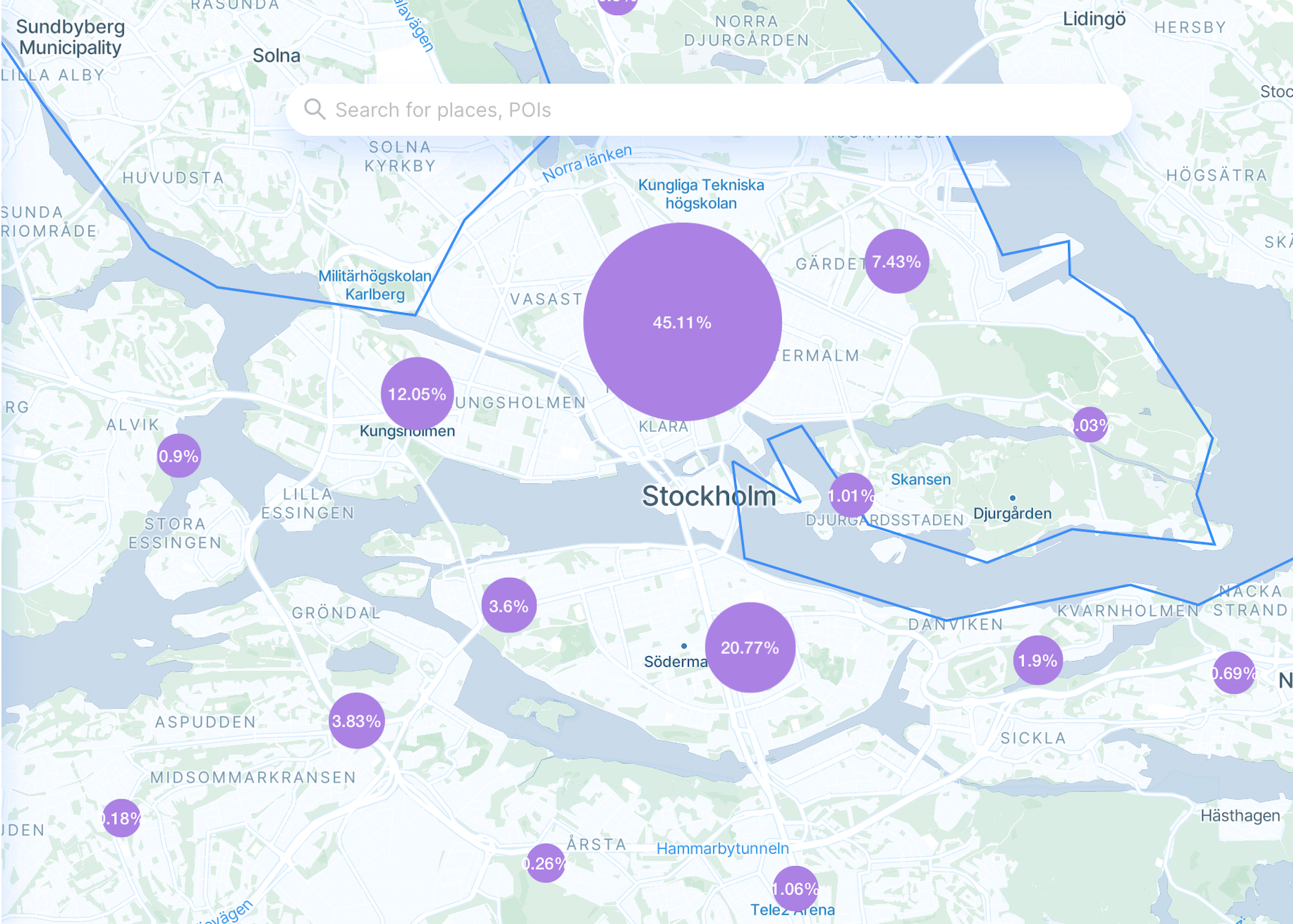
Clusters

A cluster map shows the density of events in a slightly different way. Cityscope again takes a random sample of no more than 15,000 points and displays them in bubbles. The percentages on the cluster represent the share of the sample that are present in the bubble- for example, in the image below, more than 45% of the sample points are present in the large bubble in the center.

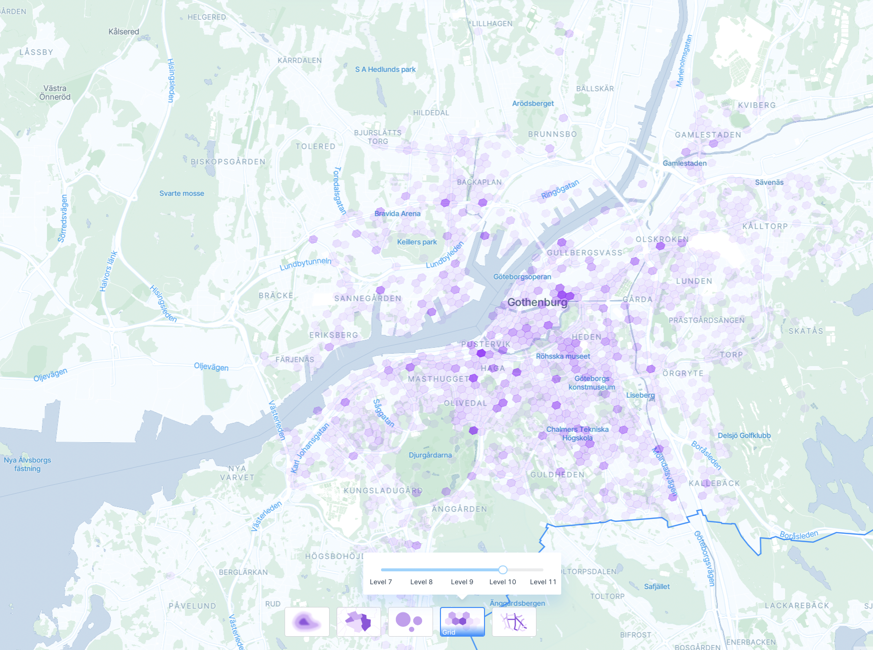
Hexes

Vianova uses the H3 system popularized by Uber to display information, especially when there data may straddle multiple political boundaries like districts and subdistricts. Cityscope again takes a random sample of data, and buckets the points into different hexes- the darker the hex, the higher the number of points.

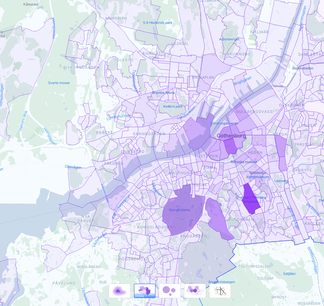
Zones

Unlike heat maps, clusters, or hexes, the "Zones" view in Activity represents real, calculated values, not samples. This fact is because Vianova has already calculated the value of every metric in every zone (district, subdistrict, custom zone, etc), every hour. Therefore, we are able to calculate the value in the same way that we produce data on the left hand side of the Activity page.

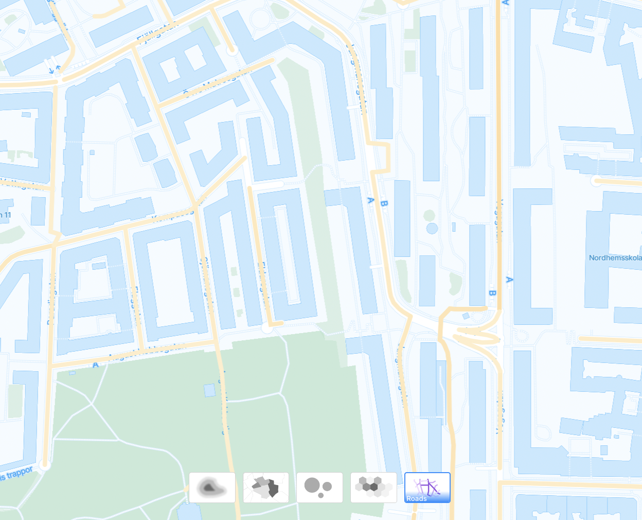
Roads

Similar to zones, Vianova calculates the number of events (parked devices, trips using the road) for every road segment in the network. This fact means that the Roads view also represents a real, calculated value for the period, and not a sample.

When working with both samples and calculated values, it is important to consider the way that time can distort the values. A single number (whether derived from a sample or a calculated value) can sometimes not be the best way to understand a long period of time. For example, over a year-long period, the number of devices parked in an area can vary wildly as a result of seasonal effects, changes in supply and demand, new transport patterns, or other effects. It is often better to look at a point over multiple, smaller increments of time, than using "one number" for a very long period of time.

More Information and SLIs

Vianova Maintains a "Feed Quality Report" which ranks certain components of a feed. You can review the current metrics here.